Data Center Cost Model Spreadsheet Structure and Limitations

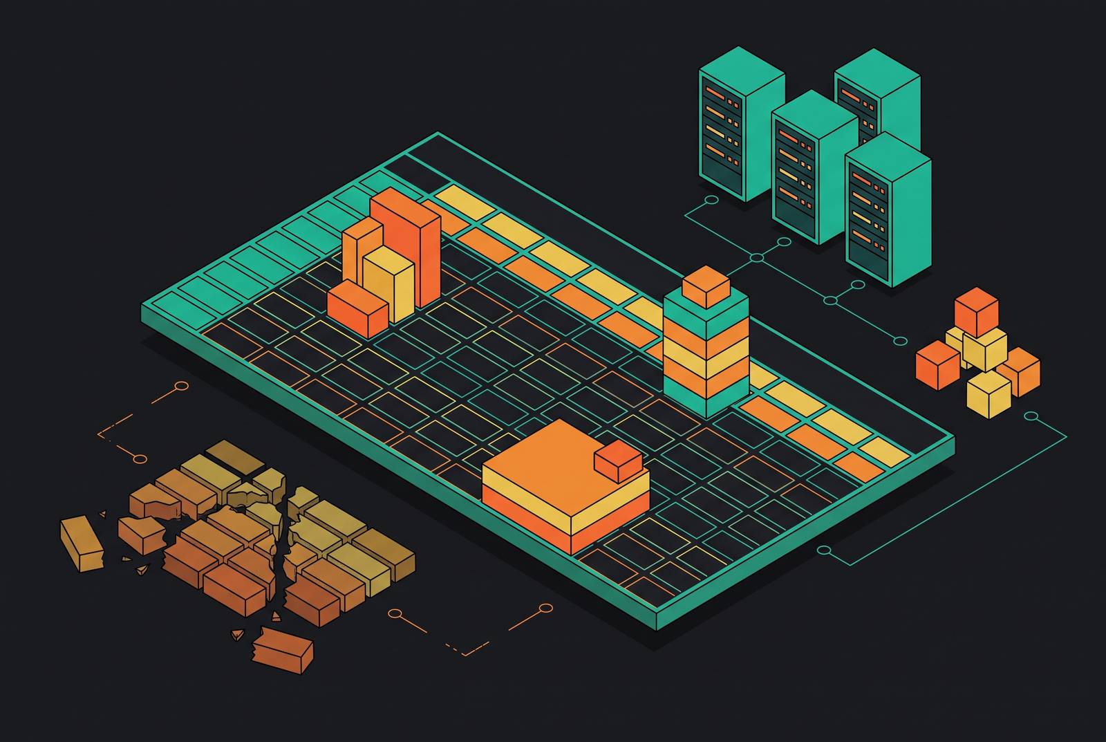
A data center cost model spreadsheet gives spending a clear structure, but that structure is not a complete model of the facility. Those limits grow as hardware lifespans get shorter, AI workloads change the inputs, and design decisions depend more on each other. The spreadsheet is useful for explaining costs and assumptions, and those costs depend on design data for their credibility.

Why the spreadsheet became the default cost model for data centers

The spreadsheet fits the top level of data center economics unusually well. Costs fall into distinct categories, including servers, facility, network infrastructure, energy, taxes, maintenance, labor, land, and water. Epoch AI’s publicly available 1 GW TCO model uses those categories, giving readers a recognizable map of total cost of ownership. A common unit such as $/kW then makes unlike expenses comparable. Once every category has a row and every row uses the same unit, the format seems to cover what is needed.

That confidence had a reasonable foundation. Construction costs changed little, new server generations came slowly, and it was clear how long facilities would last compared with the equipment inside them. A facility depreciated over a decade-plus while servers were replaced over a few years. The model could spread the cost of each purchase across its useful life and list ongoing expenses beside it. This was a practical way to compare costs that otherwise sat on different clocks.

James Hamilton’s foundational cost model made that comparison through a monthly bill. It amortized capital and billed consumables by the month, so the costs of facility investment, servers, and power could be compared on the same footing. That basic architecture still underlies most models in use today. Its appeal is not just familiarity, but a clean way to explain where the money goes.

What a standard data center cost model spreadsheet actually contains

A standard model has five layers, namely capital expenditure categories, operating expenditure assumptions, asset-life schedules, sensitivity tables, and a total cost summary. The CapEx layer separates servers, facility construction, network infrastructure, land, and utility works such as substations. Epoch AI’s 1 GW AI facility model assigns the large majority of up-front capital to servers and the facility together. The OpEx layer covers energy, maintenance, labor, taxes, and water. Energy is the largest single operating category, with its cost driven by electricity price, power usage effectiveness, or PUE, and utilization.

The amortization layer assigns a useful life to each asset class and turns its purchase cost into an annual expense. Epoch AI’s model uses 5 years for IT equipment and 14 years for the facility. It also shows how shortening IT lifespan to 3 years raises annual cost, while extending it to 7 years lowers it. Hamilton’s earlier model used amortization periods of 10 to 15 years for the data center and roughly three years for servers. Both models allow for equipment to be bought more than once during a facility’s life.

Sensitivity tables change inputs such as PUE, utilization, electricity cost, and sometimes server lifespan. Epoch AI’s model blends state-level industrial electricity rates using data center project counts from Aterio. An assumptions tab keeps these choices in one place, along with the server type and the life of the equipment. The summary then expresses TCO as an annualized cost per megawatt, subject to the selected facility design, location, financing, and power strategy.

How the amortization mismatch breaks the model before it is even run

The first structural weakness is the attempt to represent changing equipment cycles with a single useful-life assumption. A physical facility is amortized over 15 to 20 years, while AI accelerators arrive in new generations every 12 to 18 months. A new generation makes a fixed lifespan assumption carry a great deal of uncertainty while leaving the replacement timing of installed equipment undetermined. The annualized result can therefore look precise before its most consequential premise has been settled.

Epoch AI’s model shows the scale of that uncertainty. Moving between a 3-year and a 7-year IT lifespan changes annualized cost by billions of dollars per year for a 1 GW facility. At that scale, the sensitivity range largely determines the answer. Hamilton’s model shows why servers make up most of the costs at scale: they are bought again and again during the facility’s life.

Experienced modelers already test several lifespans, but a lifespan-only sensitivity table leaves the rest of the design fixed. The server type, cooling mode, and power distribution topology may all change at the same time. Epoch AI’s model assumes all servers are NVIDIA GB200 NVL72 systems, a choice that materially changes cost per MW relative to prior-generation configurations. A model built on different server assumptions may therefore be stale even if its arithmetic is sound. Even with more rows, the model still treats changes that depend on each other as separate choices.

Why AI-workload cost variables sit outside the benchmarks most models were built on

Even a better treatment of equipment life would leave a second problem, which is the benchmark gap. AI-optimized facilities differ sharply from the cloud-era facilities behind many spreadsheet defaults. Global benchmark data for AI-workload construction is not yet available at the depth needed to anchor those inputs. A familiar cost category can remain valid while the number assigned to it no longer describes the intended facility.

Turner & Townsend’s 2025 index shows a material average cost premium for liquid-cooled facilities in the US over air-cooled builds of similar IT capacity. To account for that cost difference reliably, the affected line items in an air-cooled template need new assumptions as well as a new label. WUC Technologies’ 2026 report also shows that AI workloads consume multiple times the power per rack of traditional enterprise compute. A conventional rack-density assumption can therefore understate cooling infrastructure, power distribution, and energy costs together.

Electricity benchmarks create a similar false sense of comparability. WUC Technologies’ 2026 report shows effective rates in constrained markets running materially higher than the blended national figure, with grid availability wait times of multiple years in the tightest markets. Its report also shows that OpEx makes up more of lifecycle TCO than it did several years earlier because of energy prices, more complex cooling, and the costs of specialized labor. These are changes in the cost structure. A model calibrated to older ratios can misrepresent where lifetime spending will fall.

The system-level dependency problem that no static model captures

Beyond questionable inputs lies a harder limitation. A spreadsheet separates expenses into line items, while a working AI cluster depends on a chain of equipment and decisions. Available accelerators are not installed compute without matching HBM, host servers, network fabric, optics, racks, liquid-cooling equipment, power distribution, firmware, and commissioning. A project can have GPUs on hand and still lack a working cluster. A list of what each component costs leaves out the order in which the parts must come together for the whole system to work.

Two halls with identical IT megawatts can place different demands on individual rows, electrical branches, and cooling loops. An average across the hall hides those differences. The cost of cooling capacity thus depends on the total load, the actual rack layout, and the workload profile expected in the hall. The location of that load matters as much as its sum.

Cooling choices also reach into decisions that look separate in a cost sheet. Rear-door chillers and liquid-to-chip solutions have thermal and mechanical constraints that limit how cables can be routed and which connectors can be used. Those relationships must be resolved in the design model before their costs can be extracted. A contingency percentage can reserve money for uncertainty, but it cannot identify which dependency is likely to cause an overrun or by how much. That makes contingency a financial allowance.

What breaks at handoff when the cost model and the design model never talked to each other

The separation between cost and design does not end when construction does. If cost data lives in a spreadsheet and design data lives in a BIM model without a shared structure, operations inherits the gap. Detailed geometry alone does not make an operational digital twin. A model that shows design intent but has yet to be checked against as-built conditions is still a visualization tool. Its value in operations depends on how the underlying data was organized during the build.

This becomes a practical problem at the handoff from BIM to DCIM. Schema alignment and a shared plan for asset identifiers need to be in place before construction starts. Retrofitting that connection after handover is significantly more expensive and rarely complete. Fragmented contractor spreadsheets make the problem worse when they hold critical MEP and liquid cooling data. The facility may be ready for turnover while its asset information is not.

Trimble’s H2 2025 data center trends analysis says that 95.5% of construction data is typically lost at handover. It also states that operations teams spend the first 6 months of a campus lifecycle scavenging for asset information. Stale or incomplete inventory can then leave DCIM producing inaccurate capacity reports, misleading alerts, and change records that diverge from reality. The cost model can be the earliest break in that chain if its categories never align with the asset identifiers operations requires. The mismatch then propagates beyond the estimate into the systems meant to manage the facility.

What a connected design-and-cost workflow does differently

The alternative is a different relationship between design and cost. Layout, equipment parameters, power and cooling coordination, and costs remain connected so that a change in one can flow through to the others. Rack layout, cooling loop placement, and cable tray routing are resolved in the design model first. Costs are extracted from that coordinated design second.

Disconnected project platforms make that sequence difficult to maintain. When the general contractor works in one platform and a key mechanical subcontractor works in another, changes require someone to re-enter data. The spreadsheet gives people a common format for sharing data, but it keeps cost and design apart. Each time someone transfers data by hand, cost data has another chance to fall behind design decisions. A connected workflow removes the need to translate the data each time, along with the need for people to take more care when doing it.

ArchiLabs Studio connects layouts, power and cooling coordination, cable routing, documentation, RFIs, and operations-ready handoff within a single workflow. A rack move that would otherwise require manual rework across power, cooling, cables, and sheets instead propagates automatically. Structuring BIM data from the start around DCIM, EPMS, and BMS asset identifiers also lets cost categories map to the records operations will use.

How to read a data center cost model spreadsheet knowing its limits

Start with the assumptions tab. PUE, utilization, electricity price, server type, IT lifespan, and facility lifespan are the model’s substance. Check them against the actual facility type, location, and workload profile. If you accept the defaults without that check, you take someone else’s assumptions about their facility as your own.

Check facility type first, because an air-cooled cloud benchmark will misprice an AI-optimized liquid-cooled build before the finer adjustments begin. Turner & Townsend’s 2025 index provides typology-specific benchmarks for replacing inappropriate defaults. Then treat IT lifespan sensitivity as a range of plausible scenarios rather than a refinement around a preferred base case. A range that moves annual costs by billions deserves to be presented as a central result.

Before accepting a major cost figure, trace the design decisions beneath it, including rack layout, cooling type, and power distribution topology. Check whether those decisions are settled or could still change. A figure resting on an unfixed design decision is a placeholder. Apply the same test forward into operations by mapping cost categories to the asset identifiers that DCIM, EPMS, and BMS will use. If a line item cannot be traced to an operational asset record, the model is still a financial exercise with a handoff problem attached.

Used this way, the spreadsheet gives developers, engineers, and capital partners a shared way to talk through costs and bring assumptions into view. Its legitimate role is as a communication framework, and its illegitimate role is as a substitute for a connected design model that supplies costs from live data.